Scraping Wikipedia Tables from Lists for Visualisation
Jan 30, 2018 · 2050 words · 10 minutes read
Get WikiTables from Lists
Recently I was asked to submit a short take-home challenge and I thought what better excuse for writing a quick blog post! It was on short notice so initially I stayed within the confines of my comfort zone and went for something safe and bland. However, I alleviated that rather fast; I guess you want to stand out a bit in a competitive setting. Note that it was a visualisation task, so the data scraping was just a necessary evil. On that note.
I resorted to using Wikipedia as I was asked to visualise change in a certain x going back about 500 hundred years. Not many academic datasets go that far, so Wiki will have to do for our purposes. And once you are there, why only visualise half a millennium, let’s go from 1 AD to present day. First, we need a subject. I went with my PhD topic, war duration. So let’s get the list of lists first using rvest:
#Get wikipedia time periods for List of Wars
url <- "https://en.wikipedia.org/wiki/Timeline_of_wars"
periods <- url %>%
  read_html() %>%
  html_nodes("ul") %>%
  html_text(trim = TRUE) %>%
  strsplit(split = "\n") %>%
  unlist()
periods <- periods[18:26]
periods[1] <- tolower(gsub(" ", "_", periods[1]))
periods
## [1] "before_1000" "1000–1499" "1500–1799" "1800–99"
## [5] "1900–44" "1945–89" "1990–2002" "2003–10"
## [9] "2011–present"I explained the basics of rvest in my Game of Thrones post, so I won’t go over it again. The periods vector looks good, but not really: the timeframes themselves are lists; e.g. 1800-99 actually consists of ten tables. If we run a loop, we will only get the first table of each timeframe. I would know, that’s what I got in my first attempt. Jesus, so many missing years, Wikipedia.
We need to construct an indicator to guide the loop at each timeframe. I didn’t do this programmatically, and I would be happy to know how, but I just entered the number of tables per timeframe manually in a sequence:
tables <- c(3, 1:6, 1:3, 1:10, 1:3, 1:5, rep(1, 3))
sequences <- c(periods[1],
               rep(periods[2], 6),
               rep(periods[3], 3),
               rep(periods[4], 10),
               rep(periods[5], 3),
               rep(periods[6], 5),
               periods[7:9])
tables
## [1] 3 1 2 3 4 5 6 1 2 3 1 2 3 4 5 6 7 8 9 10 1 2 3
## [24] 1 2 3 4 5 1 1 1sequences## [1] "before_1000" "1000–1499" "1000–1499" "1000–1499"
## [5] "1000–1499" "1000–1499" "1000–1499" "1500–1799"
## [9] "1500–1799" "1500–1799" "1800–99" "1800–99"
## [13] "1800–99" "1800–99" "1800–99" "1800–99"
## [17] "1800–99" "1800–99" "1800–99" "1800–99"
## [21] "1900–44" "1900–44" "1900–44" "1945–89"
## [25] "1945–89" "1945–89" "1945–89" "1945–89"
## [29] "1990–2002" "2003–10" "2011–present"Now, we can pass the base url in a loop using the above:
#Create a loop for extracting all wars since 1AD
baseurl <- "https://en.wikipedia.org/wiki/List_of_wars_"
all.wars <- NULL

for (i in 1:length(sequences)) {
  url <- paste0(baseurl, sequences[i])
  webpage <- read_html(url)
  wars <- webpage %>%
    html_nodes(xpath = paste0('//*[@id="mw-content-text"]/div/table[', tables[i], ']')) %>%
    html_table(fill = TRUE)
  all.wars[i] <- list(wars)
}

#All wars as a dataset
df <- ldply(all.wars, data.frame)
df <- df %>% arrange(Start)
Data Clean-Up and Feature Engineering
Welcome to the world of uncurated data, so let’s clean it up. First, there are some internal Wikipedia inconsistencies, so we will move columns around. Then, we will extract the first set of digits to get rid of the likes of ‘c1660, 1922(armistice), 1860s’ etc. Finally, we will drop the NAs and recode ongoing wars to 2018:
#Clean up Wikipedia inconsistencies
df$Name.of.Conflict <- ifelse(is.na(df$Name.of.Conflict),
                              df$Name.of.conflict, df$Name.of.Conflict)
df$Finish <- ifelse(is.na(df$Finish), df$Finished, df$Finish)

#Extract first set of digits as dates
df$Start <- stri_extract_first(df$Start, regex = "\\d+")
df$Finish <- stri_extract_first(df$Finish, regex = "\\d+")

#Drop NAs and correct starting dates
df <- df[, 1:5]
df <- df %>% arrange(Start)

#Correct finish dates
df$Start <- as.numeric(df$Start)
df$Finish <- as.numeric(df$Finish)
df <- df[!is.na(df$Start), ]

#Change ongoing to 2018 finish
df$Finish <- ifelse(is.na(df$Finish), 2018, df$Finish)
glimpse(df)
## Observations: 2,117
## Variables: 5
## $ Start <dbl> 1008, 101, 1010, 1014, 1015, 1018, 1018, 1019...
## $ Finish <dbl> 1008, 102, 1011, 1014, 1016, 1018, 1019, 1019...
## $ Name.of.Conflict <chr> "Hungarian–Ahtum War", "First Dacian War", "S...
## $ Belligerents <chr> "Kingdom of Hungary", "", "Liao Dynasty", "Mu...
## $ Belligerents.1 <chr> "Voivodship of Ahtum", "", "Goryeo", "Leinste...Better. Still, we don’t have that many interesting variables in there. Most of my research focuses on the distinction between interstate and civil wars, especially how they differ in their average duration over time. We can programatically identify civil wars using an arbitrary criteria with text analysis. Below, I use quanteda to accomplish the task:
#Programmatically identify civil wars using text analysis
#Define arbitrary civil war words
intrastate <- c("Revolt", "Rebellion", "Civil", "Insurgency", "Interregnum", "Uprising")
df.corpus <- corpus(df[, 3])
df.tokens <- tokens(df.corpus, what = "word")

#Identify rows that include civil war words in title
civil.wars <- tokens_select(df.tokens, pattern = intrastate, selection = "keep")
indicator <- as.data.frame(unlist(civil.wars))

#Extract row numbers as digits and only keep the first four
indicator$row <- substr(gsub("[^0-9]", "", rownames(indicator)), 1, 4)

#Drop duplicates
indicator <- distinct(indicator)
rownames(df) <- 1:nrow(df)
df$Civil.War <- ifelse(rownames(df) %in% indicator$row, 1, 0)
df$Civil.War <- as.factor(df$Civil)
df$`War Type` <- ifelse(df$Civil.War == 0, "Interstate", "Civil War")
Now that we are here, might as well include duration:
#Create a duration variable (years)
df$Duration <- (df$Finish - df$Start) + 1

#Create century indicator based on start year
df$Century <- as.integer(df$Start / 100) + 1
df$Century <- paste0(df$Century, ifelse(df$Century == 2, "nd Century",
                                        ifelse(df$Century == 3, "rd Century",
                                               ifelse(df$Century == 1 | df$Century == 21,
                                                      "st Century", "th Century"))))
df$Century <- as.factor(df$Century)
#Reorder levels from 1st to 21st
df$Century <- factor(df$Century, levels(df$Century)[c(11, 14:21, 1:10, 12:13)])
#Need this for later
df$Quarter <- ceiling(df$Start / 25)
Okay, so far we have collected information on conflict name, belligerents, start and end years, duration, century, and quarter. We can still create more from our existing data. Wikipedia, where applicable, (for the lack of a better word) codes belligerents as victorious and defeated. Meaning, if we extract the names of Side A and Side B over time, we might be able to capture the patterns of who ‘won’ and ‘lost’ in the last two thousand years. 1 I only include the code for the winners below and do the same for the defeated parties under the hood:
#Commonalities of belligerents by century
#Pool text for winners
victors <- df$Belligerents
victors <- gsub("\n", " ", victors)

#Group by century and identify most frequent words
dfm.vic <- dfm(corpus(victors, docvars = data.frame(Century = df$Century)),
               remove = stopwords("SMART"), remove_numbers = TRUE,
               remove_punct = TRUE, groups = "Century")
vic.top.words <- topfeatures(dfm.vic, n = 5, groups = docnames(dfm.vic))

#Transform list to dataframe
vic <- as.data.frame(unlist(vic.top.words))
vic$Century <- sub('\\..*', '', rownames(vic))
vic$Word <- sub('.*\\.', '', rownames(vic))
vic$Side <- "Victorious"
colnames(vic)[1] <- "Count"
Now we combine them together and create our second dataset:
#Combine and clean up
sides <- rbind(vic, def)
rownames(sides) <- 1:nrow(sides)
sides$Count <- log2(sides$Count) + .1
sides$Count <- ifelse(sides$Side == "Victorious", -sides$Count, sides$Count)
sides$Century <- as.factor(sides$Century)
sides$Century <- factor(sides$Century, levels(sides$Century)[c(11, 14:21, 1:10, 12:13)])
sides <- sides %>% group_by(Century, Word) %>% mutate(Duplicate = n() - 1)
sides$Word <- ifelse(sides$Duplicate == 0, sides$Word, paste0(sides$Word, "(", tolower(substr(sides$Side, 1, 3)), ")"))
I convert the count value for the victorious side to negative after taking its log for plotting purposes.
Visualise Actor Characteristics
Okay, fun part. Also, note that we need all that code to get the data and clean it up while the visualisations are maybe one little chunk of code. Anyway, the first visualisation I had in mind is the one I used for my Weinstein effect post. In my head-cannon, I call it the ‘tidytext difference chart’, but I’m sure there’s a proper name for it. One thing I couldn’t figure out was achieving perfect sorting; not sure what causes that (e.g. Byzantine in the 9th Century, Khaganate in the 10th century etc.). Twitter solved it!
#Requires devtools::install_github("dgrtwo/drlib")
ggplot(sides, aes(reorder_within(x = Word, by = Count, within = Century), Count, fill = Side)) +
  scale_x_reordered() +
  facet_wrap(~Century, scales = "free_y") +
  geom_col() +
  coord_flip() +
  scale_y_continuous(labels = c("12X", "", "8X", "", "4X", "", "",
                                "", "4X", "", "8X", "", "12X"),
                     breaks = seq(-6, 6)) +
  geom_hline(yintercept = 0, alpha = .4) +
  theme(legend.position = c(.5, .05)) +
  labs(title = "Who Participates in Organised Violence: Change in Actor Characteristics 1 AD-2018 AD",
       subtitle = "Five Most Common Descriptors based on Wikipedia Conflict Names | Stratified by Belligerent Type | Clustered by Century",
       caption = "@gokhan_ciflikli | Source: Wikipedia",
       x = "Most Frequent Words",
       y = "Logarithmic Scale") +
  guides(fill = guide_legend(reverse = TRUE))
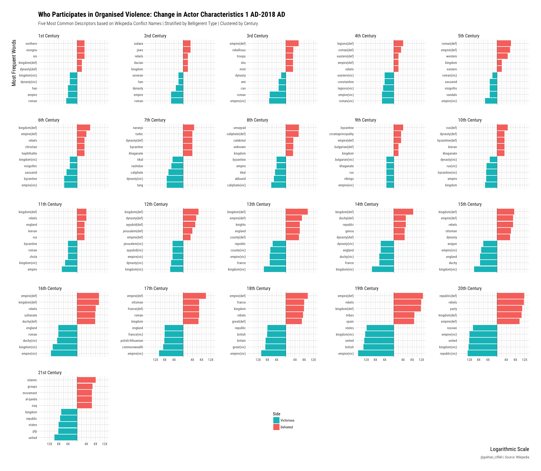
It’s not low-resolution friendly so click here. Even though Wikipedia is not an academic source and the findings should be taken with a grain of salt, the visualisation captures what we would expect to see in terms of the evolution of armed conflict over the last two millennia in terms of actors and outcome. Romans and Chinese dynasties dominate the first five centuries, followed by the Germanic tribes and Muslim empires in the following 500 years. From the 11th century onwards, we begin to see major European powers and parties associated with the Crusades. In the next five centuries (16th-20th), we witness the fall of the Ottoman Empire and serial defeats of the ‘rebel’ factions. Finally, the 21st century (only 17 years of data) is marked by the US ‘winning’ and Islamic movements being defeated. We also see that the data can be cleaned further, e.g. the ‘unknown’ faction in the 8th century.
Average Conflict Duration
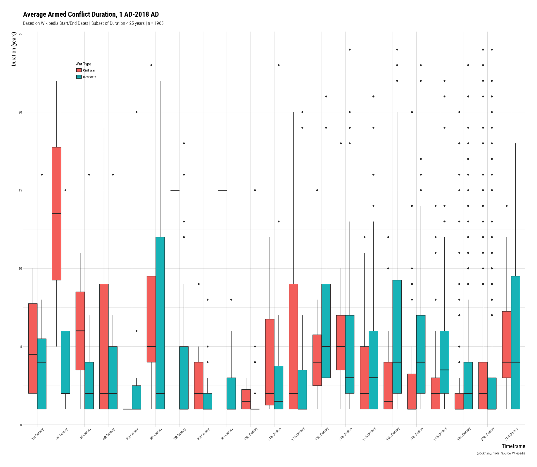
Although we differentiated between interstate and civil wars using an arbitrary selection of terms, it could still be interesting to plot their average durations over centuries. A good old box-plot will do nicely. I subset the data so that it only displays conflicts that lasted less than 25 years:
#Average duration
ggplot(df[df$Duration < 25, ], aes(Century, Duration)) +
  geom_boxplot(aes(fill = `War Type`)) +
  labs(title = "Average Armed Conflict Duration, 1 AD-2018 AD",
       subtitle = "Based on Wikipedia Start/End Dates | Subset of Duration < 25 years | n = 1965",
       caption = "@gokhan_ciflikli | Source: Wikipedia",
       x = "Timeframe",
       y = "Duration (years)") +
  theme(legend.position = c(.125, .9),
        axis.text.x = element_text(angle = 45, vjust = .6))
Larger resolution here. With the exception of the 2nd century, which could very well be data-quality related, we kind of observe similar patterns for both types of war but sometimes with different intervals. The outliers become more prominent in the last five centuries or so as well. However, note that we transformed ongoing conflicts to an end date of 2018, so we could be picking up those towards the tail.
Temporal Variation by Century
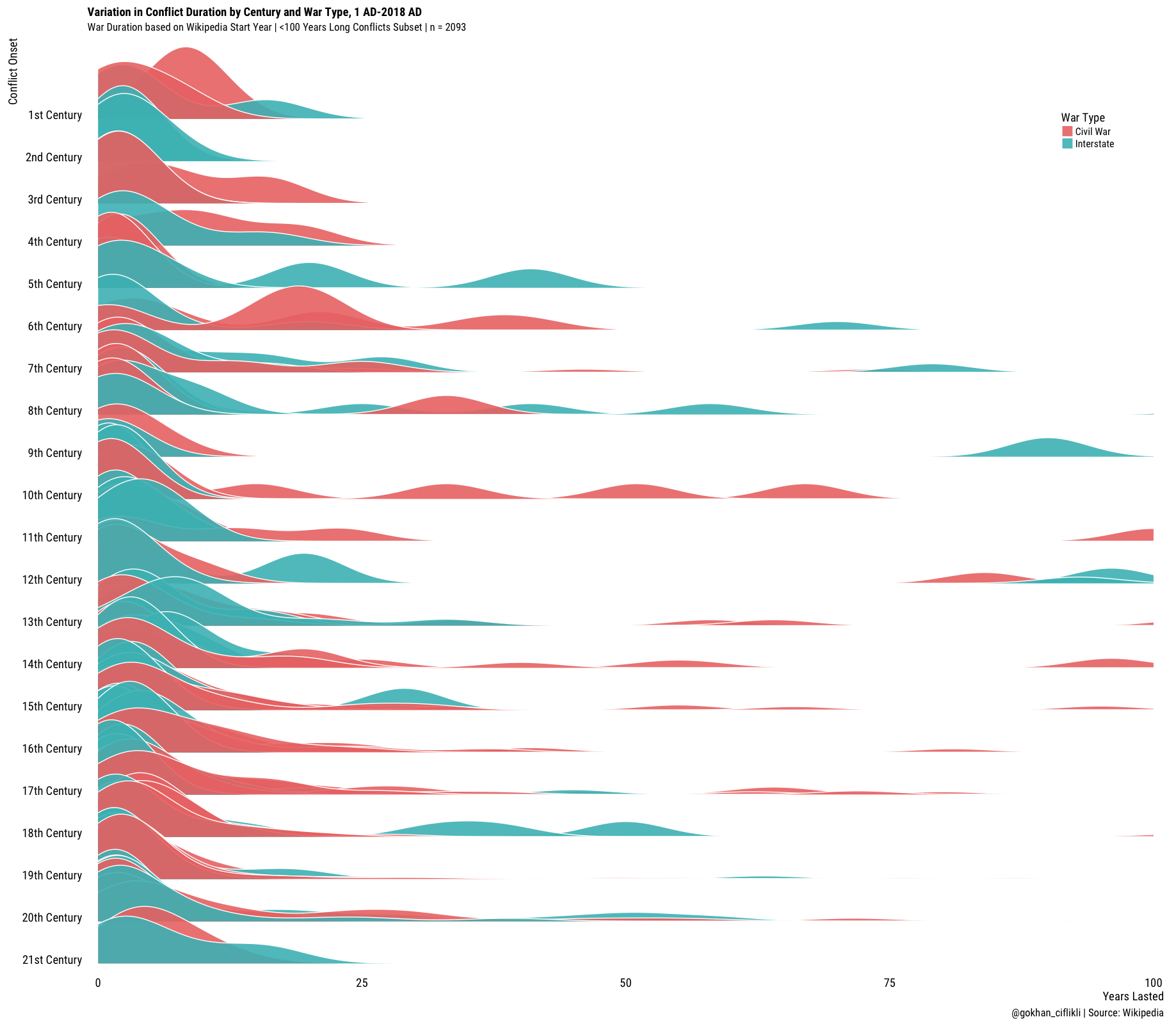
Finally, as a part of my self-issued non-viridis challenge (i.e. have a visualisation post without using viridis), I want to revisit ggridges again. We already show the important descriptives with the box-plot, so for this one I want to show, grouped by onset century, how long those conflicts lasted. I cluster the conflicts of the same type by quarter so that we have enough density in each century (otherwise some of the earlier centuries would be empty). Here it goes:
#Variation
ggplot(df, aes(y = fct_rev(Century))) +
  geom_density_ridges(aes(x = Duration, fill = paste(Quarter, `War Type`)),
           alpha = .9, color = "white", from = 0, to = 100) +
  labs(x = "Years Lasted",
       y = "Conflict Onset",
       title = "Variation in Conflict Duration by Century and War Type, 1 AD-2018 AD",
       subtitle = "War Duration based on Wikipedia Start Year | <100 Years Long Conflicts Subset | n = 2093",
       caption = "@gokhan_ciflikli | Source: Wikipedia") +
  scale_y_discrete(expand = c(.01, 0)) +
  scale_x_continuous(expand = c(.01, 0)) +
  scale_fill_cyclical(values = c("#ed7875", "#48bdc0"),
                      labels = c("Civil War", "Interstate"),
                      name = "War Type", guide = "legend") +
  theme_ridges(grid = FALSE, font_family = "Roboto Condensed") +
  theme(legend.position = c(.9, .9))
Enlarge!, a confused Picard might say in an alternate universe. On a more serious note, we find that conflicts we classify as civil wars based on their Wikipedia title have been regularly lasting more than 10+, 25+, 50+ years etc. since the 6th century. Then again, we don’t know the exact criteria for establishing the start and end dates, or even who decides what counts as conflict termination in a Wikipedia entry. With that said, feel free to experiment; code on GitHub as usual.
I quoted the terms as it is Wikipedia after all.↩